k Nearest Neighbors and related Data Structures(KD tree and LSH)

k Nearest Neighbors or aptly known as kNN is one of the most common ways to cluster similar items. In this post I'll touch on the intuition of the algorithm and some related data structures to optimize the algorithm. Related implementations in python can be found here.

Let's start with finding 1 nearest neighbour instead of k. I'll use the example of finding similar articles from wikipedia to run in conformity with the python implementations.

# 1-nearest neighbor

Say, we have a huge number of articles as our dataset. We pick one to find the articles most similar to it. Two key components are important here.

• Representation of the item i.e, articles. Word count or tf-idf can be used. TF-IDF is better for this case. Word count simply means having a dictionary that contains the count of words that appear in the article. But this is not a good choice as common words like the, and, of, to, etc will dominate. That's what makes tf-idf a better choice. TF means term frequency that is the count of a word in a particular document. IDF means inverse document frequency. That is, a measure of how commonly the word appears in other documents in the dataset. It is measured as, log(#documents / (1 + #documents the word appears in)). Then we multiply tf with idf to get a better measure of important words that are more specific to the article rather than articles and prepositions. So, that's tf-idf.

• A metric for measuring similarity or distance among the articles. There's a lot of metric for this purpose out there. Euclidean distance, cosine similarity are amongst the most common and effective ones.

So in 1-nearest neighbor, we represent the docs using say, tf-idf and then compute the distance to all other documents using a distance metric. Then return the document with the minimum distance. As easy as that.

# k-nearest neighbor

For the case of kNN, we just maintain a list of k documents that are the k nearest one's having minimum distance with our query article. We initialize our list of k nearest documents with the first k documents in sorted order. Then we compute distances for the k+1 to nth document. Whenever we encounter a document that is closer than any one of the k documents in the list, we place it in the corresponding position in the list and pop the last or kth document out of the list. At the end of the iteration, we return the list. Done!

# Caveat

Now, the approach we described is brute force. We compute distances with all the documents for each query. Each query in this approach take O(N) time for 1-NN where, N is the number of documents. For, k-NN this becomes O(Nlogk). So, when N is huge and many queries are to be performed, this approach becomes inefficient. That's what brings us to use of some more advanced data structures to make our kNN algorithm more efficient.

# KD trees

The intuition behind KD trees is simple. We take the whole data set as a rectangle box. Then cut it in smaller boxes like we cut a rectangular cake for example. So, the cuts are axis aligned. To decide where to draw the cut, we can just go down the middle like we cut cakes. Or, we can cut at the median point of the dataset along that axis. This way we can make smaller pieces of the whole rectangle. So, when we query an article, we just go the box it belongs and return the other articles in the box. Sometimes, we also check out the nearby boxes to find nearest neighbours because in the border areas, two items from two different boxes might be closer. More like what is true for border regions between countries.

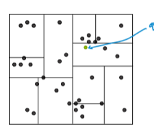
Figure: Representation of KD tree. (Photo courtesy: Emily Fox & Carlos Guestrin, ML Specialization)

# Caveat

KD trees work well for data with low dimensions. With the increase of dimensions, the data points seem to be far away from each other, so we are forced to search more boxes. Eventually, it becomes similar to brute force. So, for datasets with higher dimensions, KD tree is not the best choice. That's where the next data structure LSH comes in.

# Locality Sensitive Hashing (LSH)

In this data structure, we draw random lines that go through the origin to separate regions or boxes as opposed to KD trees where we drew lines along axes. Points that are closer to each other have a higher probability to fall in the same region when we draw lines at random. So, we draw a number of lines, how do we specify the regions? For each line, points on one side of it will yield negative results for the line's equation and positive on the other side. So, to define regions, we use 0s and 1s to denote which side it is in for a particular line. For example, let's say we have 3 lines. So, the region which is positive for all the lines will be denoted as 111 and the negative one will be denoted as 000 and the other regions will be denoted with combinations in between.

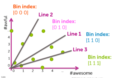
Figure: Representation of LSH. (Photo courtesy: Emily Fox & Carlos Guestrin, ML Specialization)

So, in this data structure, we retain a table or dictionary for each region. The region code is the key and the value is a list of the documents that are in that region. So, when we query a document, we find out the key for the region that it is in, then we return the other documents from the list of documents corresponding to that region. Cool, eh? We can also search nearby regions as well for nearest neighbors by just flipping the bits of the region code to search in nearby regions. We can tune the efficiency by controlling the number of regions i.e, lines and the limit for searching nearby regions. A detailed implementation of LSH can be found here.

Note: The codes are implemented as a part of assignments in the Machine Learning Specialization from University of Washington on Coursera.